
TRANSECT Manual 24.04
TRANSECT Manual 24.041. Background2. Getting started2.1 Installation using Conda2.2 Native installation on Ubuntu3. Basic demonstration4. TRANSECT workflow4.1 Prepare workflow diagram4.2 Analyse workflow diagram5. Stratification modes5.1 Single gene analysis5.2 Composite gene analysis - Additive mode 5.3 Composite gene analysis - Ratio mode5.4 Multimodal analysis6. Prepare commands and options6.1 RECOUNT36.2 GTEx6.3 GDC7. Analysis commands and options7.1 RECOUNT37.2 GTEx7.3 GDC8. Output8.1 01-Stratification8.2 02-DE8.3 03-Enrichment9. Precautions9.1 Cohort size9.2 Bulk RNA-seq heterogeneity10. Example commands11. Custom Databases11.1 Subsetting preconfigured DBs 11.2 Using private, in-house or custom data sets 12. Publication details
1. Background
TRANSECT works by defining two groups (strata, plural for stratum) within a cohort based solely on the expression of a gene or a gene set of interest and subsequently compares the stratum, one against the other, for global expression changes and functional differences. TRANSECT outputs descriptive statistics about the gene/s of interest, the products of the stratification process, the differential expression results and subsequent enrichment outcomes. The application uses publicly available large cohort datasets and simply requires the user to choose at a minimum
the cohort database containing participant IDs and gene expression measurements
a gene (or multiple genes) of interest whose expression levels are used to rank participants in the cohort database
an integer percentile value used on the expression or ranking measurements as a threshold to partition the cohort into low and high stratum for subsequent comparisons
2. Getting started
2.1 Installation using Conda
(10 - 15 minutes on an average PC)
Making use of a Conda environment for the sizable number of prerequisite modules and dependencies needed by TRANSECT is recommended for most use cases. It is not only easier to achieve but cleaner, simpler to manage and way quicker than the native install
Start by cloning the repository using the git command to a suitable location on your device
$ git clone https://github.com/twobeers75/TRANSECT.gitAlternatively TRANSECT code and executable files can be downloaded from GitHub at https://github.com/twobeers75/TRANSECT. Click on the green "Code" button followed by "Download ZIP" (note the download location). Find the downloaded ZIP file and move it to an appropriate location if required, before extracting the contents and renaming the folder
xxxxxxxxxx$ unzip TRANSECT-main.zip$ mv TRANSECT-main TRANSECTInstall Conda on your system (version > 24.1.0). You can skip this step if you already have it. There are many wikis on how to install Conda for Ubuntu, here is just one. Please consult the Conda documentation relevant to your operating system.
x### follow the instructions outlined in the link above which should look something like this for Linux$ mkdir -p ~/miniconda3$ wget https://repo.anaconda.com/miniconda/Miniconda3-latest-Linux-x86_64.sh -O ~/miniconda3/miniconda.sh$ bash ~/miniconda3/miniconda.sh -b -u -p ~/miniconda3$ rm -rf ~/miniconda3/miniconda.sh### don't forget to initialize the bash shell. Mac users need to check their default shell and change the following command appropriately$ ~/miniconda3/bin/conda init bash### Afterwards, you will be asked to restart your terminal whereby you should see (base) at the prompt. Ignore it for now.Next, we create the TRANSECT Conda environment. Here we will run an installation script that automates the creation of the TRANSECT environment, with all the tools and dependencies required to run TRANSECT. The scripts required for this can be found in the INSTALL/ subdirectory of the TRANSECT folder.
xxxxxxxxxx### change into the top directory of the downloaded folder (TRANSECT) and navigate to the INSTALL folder$ cd <path to>/TRANSECT/INSTALL### First, run the conda install script$ ./TRANSECT_conda_install.sh### Next, upon successful completion of the previous step, activate the newly created environment$ conda activate TRANSECT### Finally, whilst still within the TRANSECT/INSTALL directory and in the TRANSECT environment run the post installation script to complete the setup$ ./TRANSECT_post_conda_install.sh### You now need to reactivate the TRANSECT environment to apply the changes.$ conda deactivate$ conda activate TRANSECT
And that's it! You should now have all the necessary applications and dependencies in the TRANSECT environment to run this application. Please note, just like any virtual environment you are required to activate the TRANSECT environment in order to use the application. You can deactivate at will when not in use.
A few extra very useful commands for those not accustomed to Conda environments
xxxxxxxxxx### By default, Conda auto-activates the "base" default environment so each time you open a terminal you will automatically be in the (base) environment. I prefer not to have this happen. To disable, run the following commands. #First, deactivate any environment until there is no (XXX) at the beginning of the prompt, then turn off auto_activate_base$ conda deactivate$ conda config --set auto_activate_base false
### To check what environments you have on your system$ conda env list### You should see "base" and "TRANSECT" at the very least
### To activate TRANSECT at any time$ conda activate TRANSECT### Once you have finished, to deactivate the TRANSECT environment$ conda deactivate
### To remove/uninstall the TRANSECT environmentconda remove -n TRANSECT –all
More information about managing Conda environment can be found here
2.2 Native installation on Ubuntu
(30 - 45 minutes or longer on an average PC)
NOTE: This is not the recommended installation procedure. TRANSECT requires and depends on numerous packages and applications. These take some time to install natively if not already present. A fresh install on a vanilla Ubuntu 22.04 can take 30-45mins depending on the PC and network speeds.
To start, clone the repo
xxxxxxxxxx$ git clone https://github.com/twobeers75/TRANSECT.gitAlternatively TRANSECT code and executable files can be downloaded from GitHub at https://github.com/twobeers75/TRANSECT. Click on the green "Code" button followed by "Download ZIP" (note the download location). Find the downloaded ZIP file and move it to an appropriate location if required, before extracting the contents and renaming the folder
xxxxxxxxxx$ unzip TRANSECT-main.zip$ mv TRANSECT-main TRANSECTInstall python3 pip, java if required, and other TRANSECT dependencies (approx. 1-2min)
xxxxxxxxxx### change into the top directory of the downloaded folder (TRANSECT)$ cd <path to>/TRANSECT### install pip and other deb requirements$ sudo apt install python3-pip default-jre libfontconfig1-dev libcurl4-openssl-dev libssl-dev libxml2-dev libharfbuzz-dev libfribidi-dev libfreetype6-dev libpng-dev libtiff5-dev libjpeg-dev pandoc### install python modules$ python3 -m pip install -r pip_requirements.txtInstall R, the "pacman" package and Bioconductor specific packages. You can skip this step if you already have R. There are many wikis on how to install R on Ubuntu, here is just one (specifically for Ubuntu 22.04) (approx. 1min)
xxxxxxxxxx# follow the instructions outlined in the link above which should look something like this$ wget -qO- https://cloud.r-project.org/bin/linux/ubuntu/marutter_pubkey.asc | sudo gpg --dearmor -o /usr/share/keyrings/r-project.gpg$ echo "deb [signed-by=/usr/share/keyrings/r-project.gpg] https://cloud.r-project.org/bin/linux/ubuntu jammy-cran40/" | sudo $ tee -a /etc/apt/sources.list.d/r-project.list$ sudo apt update$ sudo apt install r-baseStart R from the terminal and install pacman and devtools. Follow the prompts and choose (if asked) to install these packages into a personal library.
Once you enter the R shell you should see printed out in the terminal a number of lines about the R version and licenses followed by a ">" symbol. I have used this symbol below to indicate that you need to be in the R shell to run these commands but, you can't copy the ">" symbol too. It won't work. *(approx. 25mins)
xxxxxxxxxx### start RR> install.packages(c("pacman","devtools"))# Note: maybe wise here to go get a coffee as the previous command takes quite some time to finish! (approx. 15mins)### whilst still in the R environment, load devtools and install rlogging> library("devtools")> install_github("https://github.com/mjkallen/rlogging.git")### also install required Bioconductor packages> if (!require("BiocManager", quietly = TRUE))install.packages("BiocManager")> BiocManager::install(version = "3.19")> BiocManager::install(c("edgeR","Glimma","DEFormats"))# Note: probably time for another coffee. Sorry! (approx. 10mins)### once successfully completed you can quit R, no need to save the workspace.# No more coffee for you today ;-)> q()
NOTE: TRANSECT requires many additional R packages however these are all installed on demand the first time (and only the first time) you run each one of the different TRANSECT commands after a nativ install. Please keep this in mind on your first run as it will take substantially longer compared to all subsequent runs.
3. Basic demonstration
TRANSECT has two main operations; Prepare and Analyse.
In order for TRANSECT to function, it first requires a cohort dataset to work on. This is retrieved and formatted appropriately by the Prepare scripts. Subsequently, TRANSECT can run analyses on the downloaded data using the Analyse scripts
Example commands to investigate ZEB1 using the RECOUNT3 TCGA PRAD cohort;
xxxxxxxxxx### First, if not already make sure to activate the TRANSECT environmentconda activate TRANSECT
### Next Download the RECOUNT3 PRAD data (approx. 3mins)# run the RECOUNT3 prepare script for TCGA-PRAD (the resulting files can be found in <path to>/TRANSECT/data/RECOUNT3/PRAD)R3_prepare_directories.sh -p PRAD# NOTE: you only need to do this one time per cohort dataset. Once you have it you don't need to download it again!
### Finally, Run the TRANSECT analysis# TRANSECT saves output in the current working folder so best to create a new folder specifically for each runcd <path to>/TRANSECT/output/RECOUNT3mkdir -p ZEB1_PRAD_testcd ZEB1_PRAD_test
# Now, run the RECOUNT3 analyse script using the PRAD data we just retreived, investigating the gene ZEB1, partitioning the participants using a percentile threshold of 5, with all outputs.R3_analyse_GOI.sh -p PRAD -g ZEB1 -s mRNA -t 5 -a
### Done! Explore the outputs. Try swapping ZEB1 for your favourite gene (remember, new folder for each run).
4. TRANSECT workflow
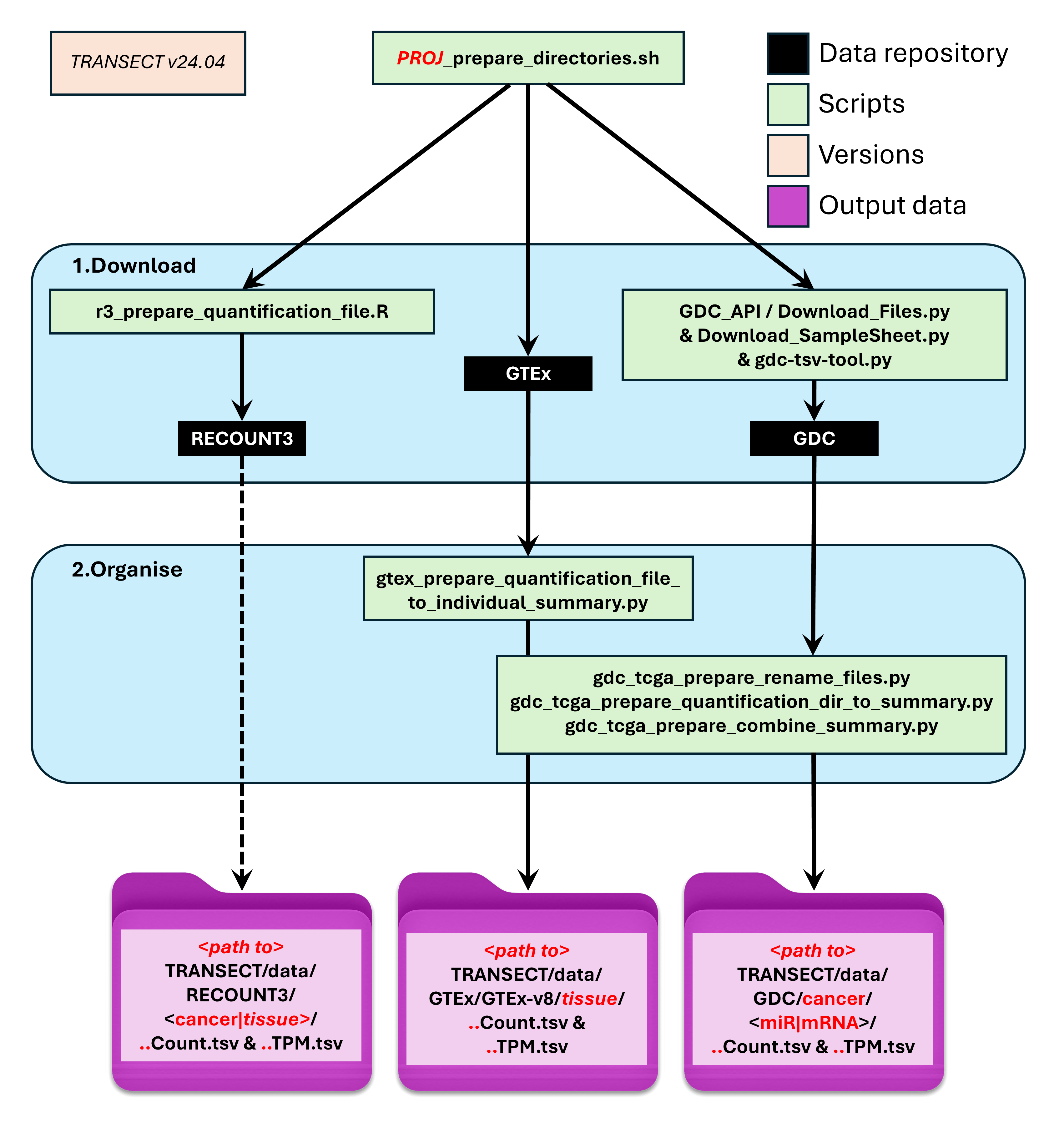
4.1 Prepare workflow diagram
4.2 Analyse workflow diagram
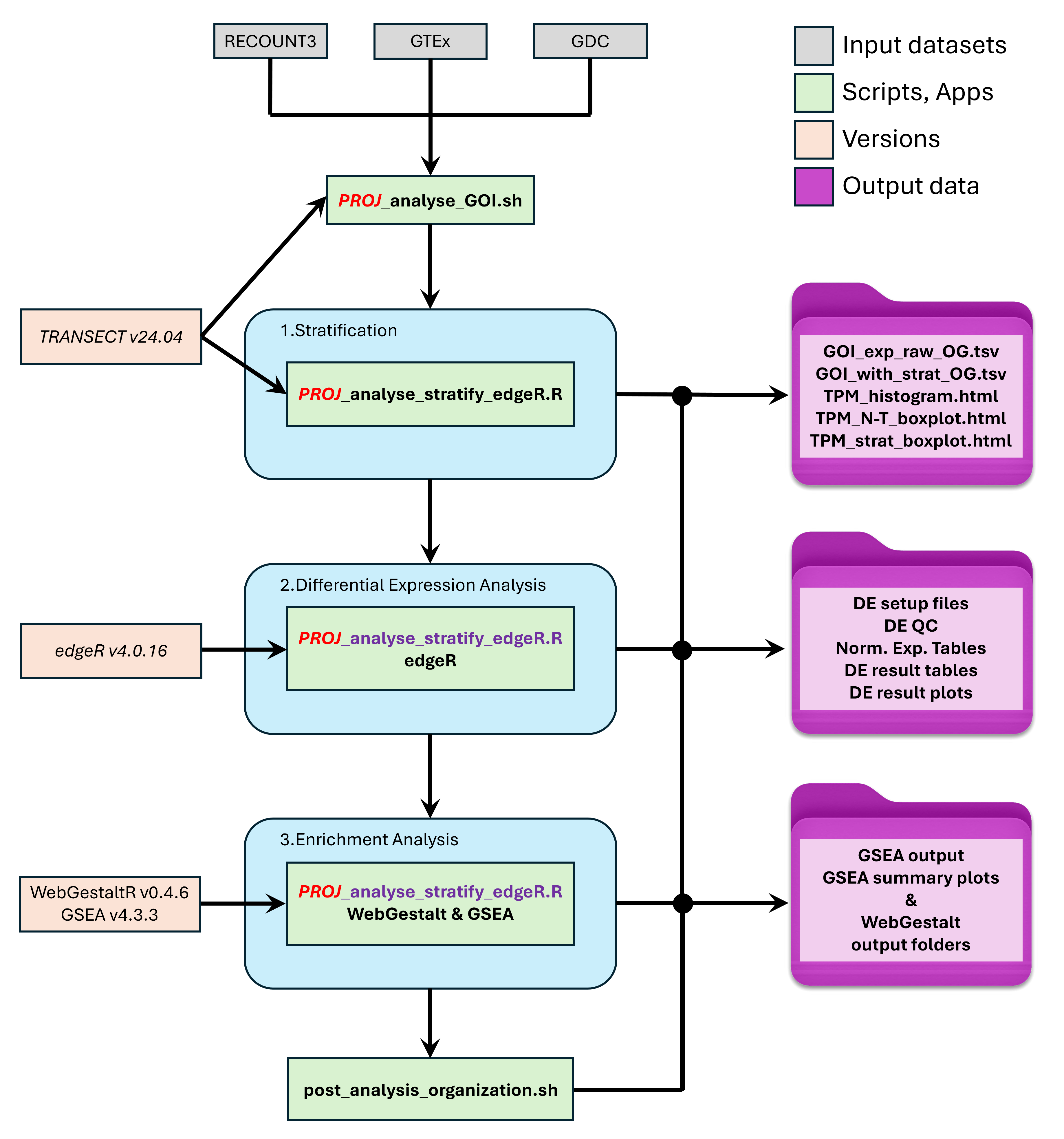
5. Stratification modes
The basic premise of TRANSECT is to stratify individuals from large cohort transcriptomic data into defined groups called strata based on singular gene expression or composite gene expression sets. The stratified participant strata are subsequently compared one to the other in order to assess global expression changes and functional differences.
5.1 Single gene analysis
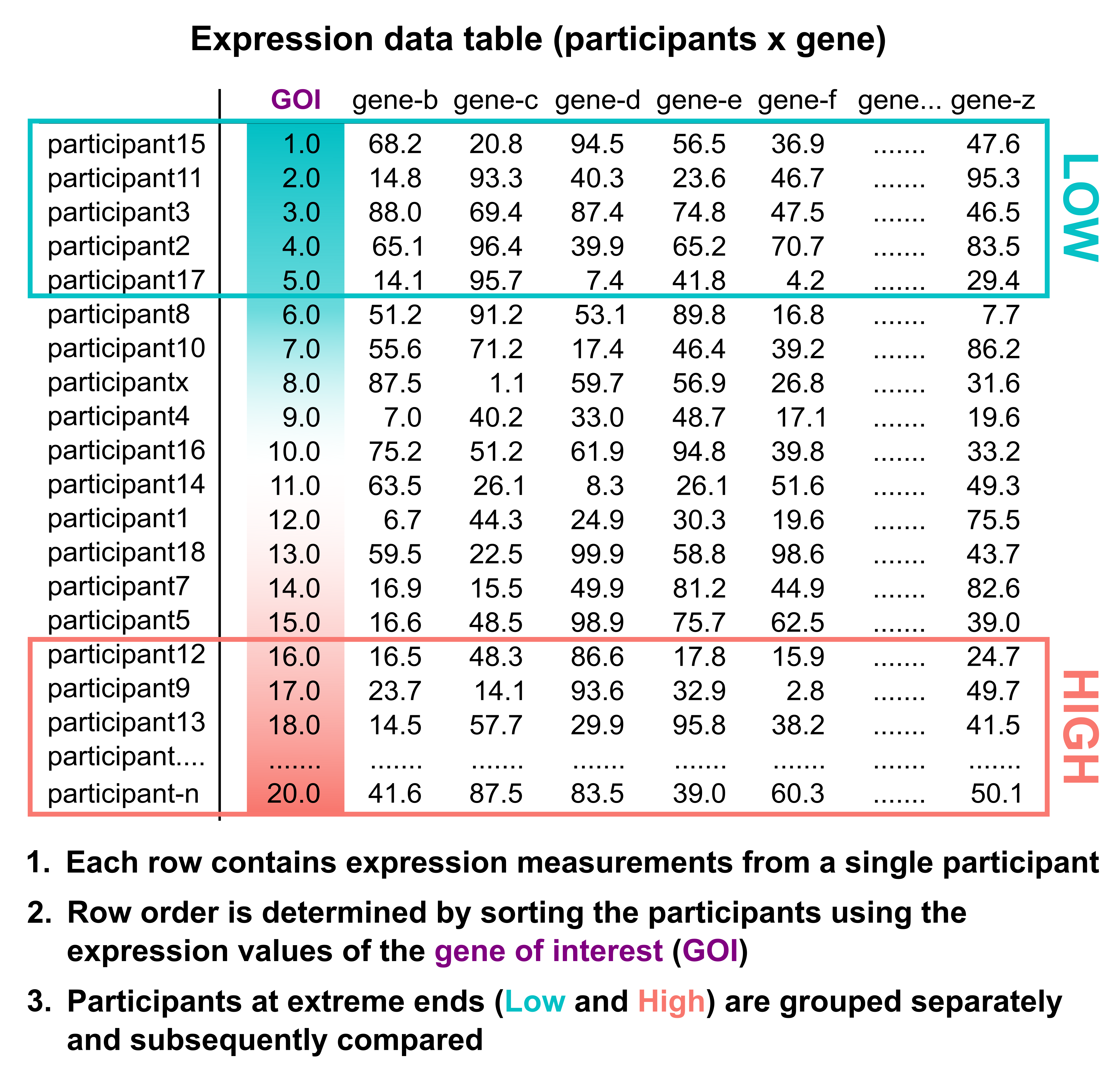
Single gene stratification is simply the division of individuals within a cohort population into distinct strata based solely on the expression of one single gene. In the current version of TRANSECT, individuals with expression levels at or near both ends of the physiological limits for the gene of interest are grouped separately and subsequently compared (depiction below).
5.2 Composite gene analysis - Additive mode
Composite analyses use information from multiple genes simultaneously to divide individuals within a cohort population into distinct strata. The additive mode of TRANSECT uses expression information from multiple genes (2 – 5 genes in the current implementation) to rank individuals expressing each of the component genes at near to physiological extreme and separate them into low and high strata for subsequent DE analysis. This is achieved by computing the average of rank positions for all component genes for each participant and using the metric to position each individual within the cohort in order. Once this is achieved and in like manner to the single gene analysis, individuals with extreme high average rank positions are grouped and compared to individuals with extreme low rank positions.
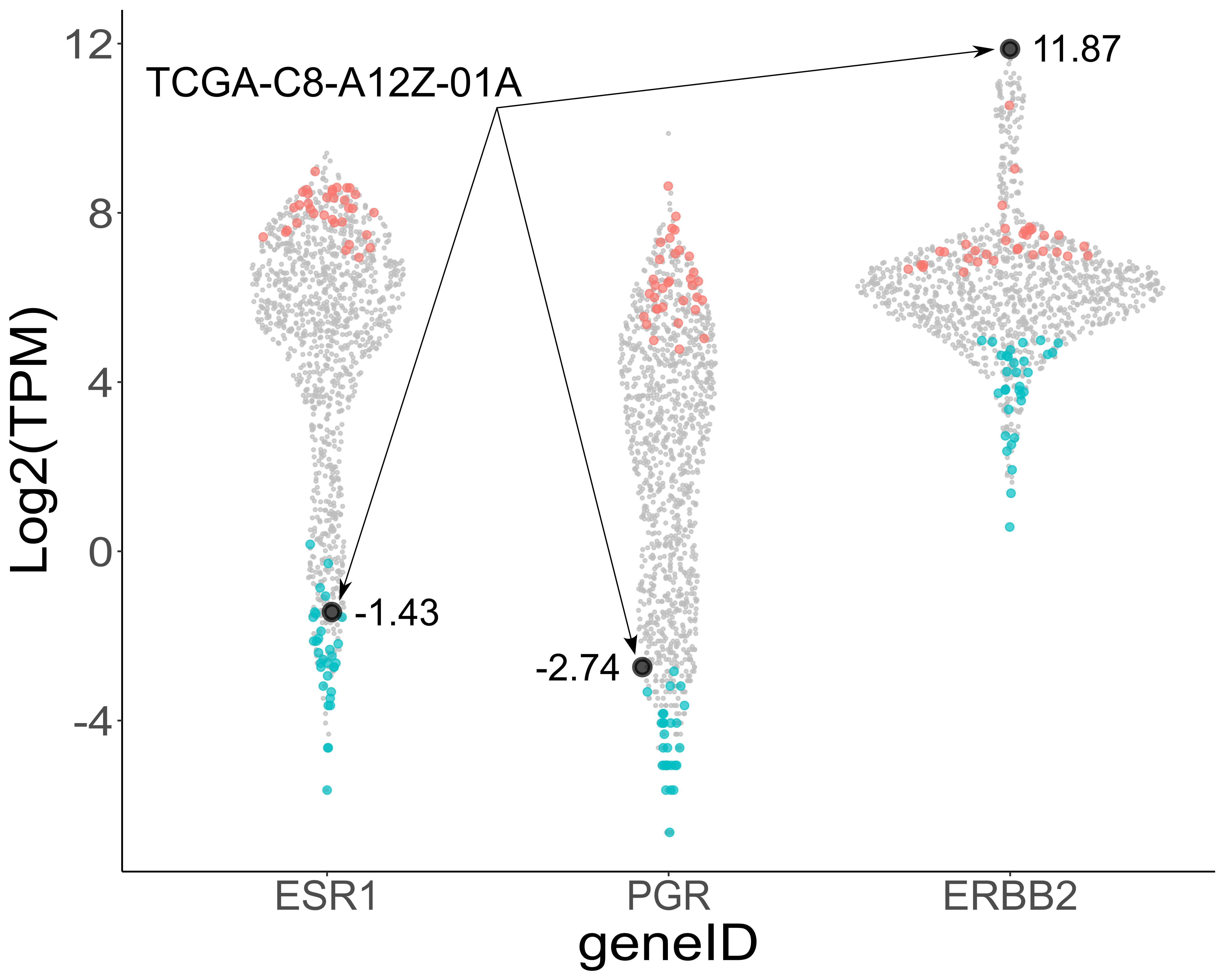
It is important to note that this process leads, in most scenarios, to the exclusion of participants with extreme expression for any one (or more) of the component genes of interest. A good example of this can be seen from the additive mode case study for ESR1, PGR and ERBB2 (triple-negative breast cancer genes) in the RECOUNT3 BRCA cohort.
The figure below (a TRANSECT output for this type of analysis), plots the expression level separately for each component gene (here ESR1, PGR and ERBB2), for each participant. Expanding on this, each participant in the cohort occupies a single point on each of the three distributions in the figure, corresponding to the participants expression level for the three genes of interest. Featured on the figure below is participant TCGA-C8-A12Z-01A who possesses the highest expression level for ERBB2 (TPM=3747.42) of all participants in the cohort however, does not express either ESR1 nor PGR (TPM=0.37 and 0.15 respectively). Individuals stratified by TRANSECT who rank low for expression of all three receptors are marked in cyan (one point per individual on each of the three distributions) and conversely, those ranking high for elevated expression of all three receptor genes are marked in magenta.
5.3 Composite gene analysis - Ratio mode
In the same manner as the additive mode described above, the ratio mode also considers information from multiple genes simultaneously to partition individuals within a cohort population into distinct strata. The ratio mode uses expression information from strictly two genes to rank individuals. In order to achieve this, TRANSECT calculates a simple log-ratio statistic (log fold change) between the 2 genes of interest for each patient and uses this as the rank metric. Extremely low ratio scores will demarcate participants where geneA >>> geneB and vice versa. Again, individuals at both extremes are grouped and compared.
Like the additive mode, participants with extreme expression for any one of the component genes may, or may not, make it in to the stratified groups for later comparison.
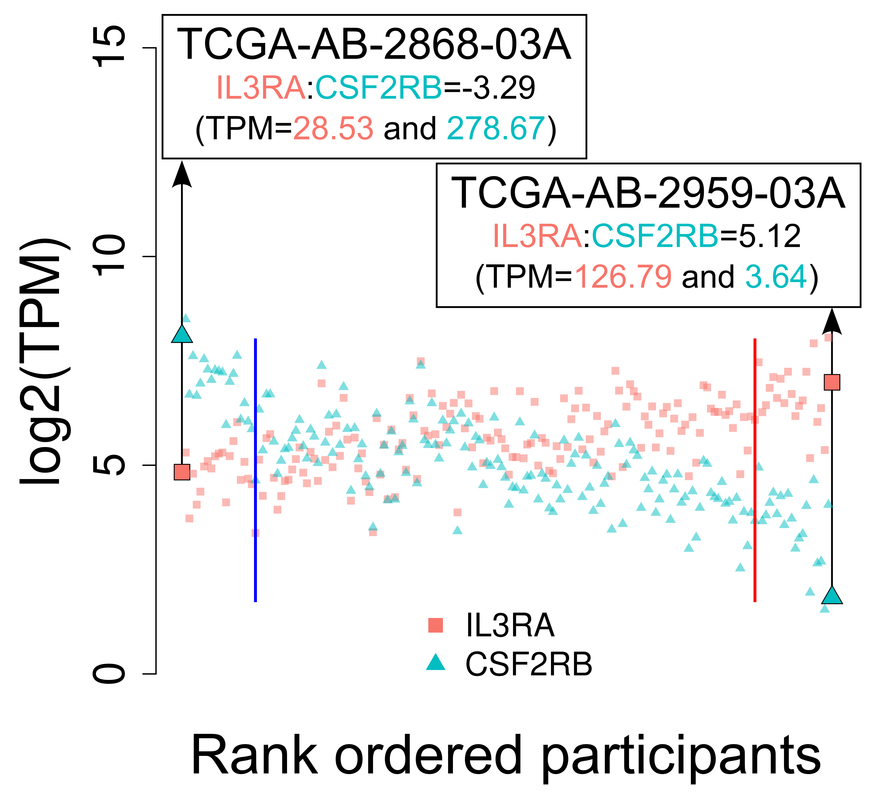
The figure below (another TRANSECT output for this type of analysis), plots the expression level separately for the two component genes (IL3RA and CSF2RB), for each participant. Expanding on this, here each participant in the cohort occupies two points on the plot (each point directly above and below the other), corresponding to the participants expression level for the two genes of interest. Participants are ordered across the x-axis from low to high based on their ratio score (converted to a rank metric). Featured on the figure below are two participants TCGA-AB-2868-03A and TCGA-AB-2959-03A who rank lowest and highest for this analysis in this cohort respectively, showing both the ratio score and TPM expression values. The solid vertical blue and red lines demarcate the thresholds for inclusion into the low and high strata respectively.
5.4 Multimodal analysis
In select large cohort studies there exist measurements derived from multiple omics for the same individual at the same or similar timepoints. For example, the TCGA study consists of RNA (mRNA, miRNA), and DNA (methylation, mutation, and copy number) data in addition to the associated global proteomics data generated by the Clinical Proteomic Tumor Analysis Consortium (CPTAC). TRANSECT has the facility to survey changes in one omics data type based on the stratification of individuals using matched data from another omics. As in the use cases above, individuals at each extreme are grouped and compared.
TRANSECT comes preconfigured with the ability to assess global changes in mRNAs based on the stratification of cohort participants based on their miRNA expression. This can only run whilst using GDC TCGA data that possess sufficient numbers of mRNA and miRNA expression data. Other types of multimodal analyses using different omics types require custom configuration.
6. Prepare commands and options
Prepare is a process that retrieves the raw data from online repositories and prepares it (if required) for analysis. TRANSECT comes bundled with three different prepare scripts, one each for RECOUNT3, GTEx and GDC-TCGA data.
All downloaded and formatted data is stored by default in the TRANSECT/data/<RECOUNT3|GTEx|GDC>/ subdirectory in individual folders named by tissue/cancer abbreviation. For example, the RECOUNT3 PRAD data downloaded in the basic demonstration of this manual is stored in
6.1 RECOUNT3
Retrieve and prepare RECOUNT3 RNA-seq data for in-house custom analyses.
USAGE:
xxxxxxxxxx$ R3_prepare_directories.sh [-h] -p <RECOUNT3 Project ID> PARAMETERS: -h Show help text -p RECOUNT3 project id: needs to be valid RECOUNT3 project id (ie. BRCA for TCGA data OR BREAST for GTEx). Required You can retrieve and prepare more than one RECOUNT dataset by using a bash for loop like this;
xxxxxxxxxx$ for r3_code in COAD BREAST LAML; do R3_prepare_directories.sh -p $r3_code ; done6.2 GTEx
Retrieve and prepare GTEx RNA-seq data for in-house custom analyses. Unlike RECOUNT3 and GDC data retrieval, GTEx data for all tissue types are retrieved in a single file. Subsequently, this is separated into tissue specific datasets using the information in the metadata file.
USAGE:
xxxxxxxxxx$ GTEx_prepare_directories.sh [-h] [-a -c -t]PARAMETERS: -h Show help text -a retrieve all expression data (mRNA counts and TPMs), Required for the proper functioning of TRANSECT -c retrieve only mRNA counts -t retrieve only mRNA TPMs
6.3 GDC
Retrieve and prepare TCGA RNA-seq data for in-house custom analyses.
USAGE:
xxxxxxxxxx$ GDC_TCGA_prepare_directories.sh [-h] -p <TCGA Project ID> [-a -c -r -R -k -n]PARAMETERS: -h Show help text -p TCGA project id: needs to be valid TCGA project id as used by GDC (ie. TCGA-BRCA). Required -a retrieve all expression data (mRNA counts and TPMs as well as miR and isomiR RPMs) -c retrieve only mRNA counts -r retrieve only miR RPMs -R retrieve only isomiR RPMs -k keep all data (Default: False) -n data is not from TCGA study (Default: False)
To retrieve and prepare more than one TCGA cancer dataset use a bash for loop like this;
xxxxxxxxxx$ for tcga_code in TCGA-COAD TCGA-SARC TCGA-LAML; do GDC_TCGA_prepare_directories.sh -p $tcga_code; doneTo retrieve and prepare all TCGA cancer datasets you can loop through all lines in GDC_API/TCGA_Study_Abbreviations.tsv (WARNING: this requires lots of time, network and disc space)
xxxxxxxxxx$ while read tcga_code; do GDC_TCGA_prepare_directories.sh -p $tcga_code; done < <(cut -f1 GDC_API/TCGA_Study_Abbreviations.tsv | tail -n +2)
Please be aware that some of these collections are large and require substantial disk space. They can take a considerable amount of time to download and process. For example, downloading and processing GDC TCGA-BRCA takes just over 30 minutes (using a high speed network connection and an up to date workstation) and requires more than 14GB of disk space (most of which can and by default is, deleted afterwards). In comparison, GDC TCGA-LAML takes less than 5 minutes to retrieve and less than 2GB of disc space.
In addition, the GDC prepare script often fails when downloading large datasets. This is caused by network connectivity issues (tested only in Australia) with the GDC repository. If you experience issues, delete the relevant dataset and retry the prepare command.
7. Analysis commands and options
Analyse is a process that uses the prepared public data from above, conducts the stratified differential expression and produces all the outputs. Like with the prepare operations, TRANSECT comes bundled with three analyse scripts, one each for RECOUNT3, GTEx and GDC-TCGA.
Unlike the prepare operations, the output from these calls is saved in the current working directory and therefore it is recommended to create a descriptively named folder for each of your analyses. TRANSECT comes with an preinstalled output folder containing subdirectories (TRANSECT/output/<RECOUNT3|GTEx|GDC>/) however, you may choose any working directory at your discretion. Keep in mind that if TRANSECT output exists in the current working directory, it will be overwritten.
For each script, composite analyses can be run using the plus charater (+) for additive combinations or by using the modulus character (%) for ratio. The two special characters are used between gene names like so. Additive example: ESR1+PGR+ERBB2 or Ratio example: ESRP1%ZEB1
7.1 RECOUNT3
Differential expression analysis of RECOUNT3 data stratified into high and low groups by gene of interest Please run this wrapper script in the directory of the desired output location
USAGE:
xxxxxxxxxx$ R3_analyse_GOI.sh [-h] -p <RECOUNT3 projectID> -g <GOI> -s <StratifyBy> -t <Percentile> -e -S -a -c -dPARAMETERS: -h Show help text -p RECOUNT3 tissue id: needs to be valid RECOUNT3 tissue id as at RECOUNT3 (ie. BRCA for TCGA or BREAST for GTEx). Required -g Gene of interest: needs to be a valid HGNC symbol (ie. ZEB1). Required -s Stratify by molecule: Must match -g and can only be mRNA at present. Required -t Percentile: startify data into top and bottom x percentile (valid x between 2 and 25). Required -e Enrichment analyses: Run GSEA on DE results (Default: Only run WebGestalt) -S Switch pairwise comparison: find genes DE in low group compared to high group (Default: high compared to low) -a Do all analyses -c Do correlation analysis only -d Do differential expression analysis only
7.2 GTEx
Differential expression analysis of GTEx data stratified into high and low groups by gene of interest Please run this wrapper script in the directory of the desired output location
USAGE:
xxxxxxxxxx$ GTEx_analyse_GOI.sh [-h] -p <GTExTissueID> -g <GOI> -s <StratifyBy> -t <Percentile> -e -S -a -c -dPARAMETERS: -h Show help text -p GTEx tissue id: needs to be valid GTEx tissue id as at GTEx (ie. Breast). Required -g Gene of interest: needs to be a valid HGNC symbol (ie. ZEB1). Required -s Stratify by molecule: Must match -g and can only be mRNA at present. Required -t Percentile: startify data into top and bottom x percentil (valid x between 2 and 25). Required -e Enrichment analyses: Run GSEA on DE results (Default: Only run WebGestalt) -S Switch pairwise comparison: find genes DE in low group compared to high group (Default: high compared to low) -a Do all analyses -c Do correlation analysis only -d Do differential expression analysis only
7.3 GDC
Differential expression analysis of TCGA data stratified into high and low groups by gene of interest Please run this wrapper script in the directory of the desired output location
USAGE:
xxxxxxxxxx$ GDC_TCGA_analyse_GOI.sh [-h] -p <TCGAProjectID> -g <GOI> -s <StratifyBy> -t <Percentile> -e -S -a -c -dPARAMETERS: -h Show this help text -p TCGA project id: needs to be valid TCGA project id as at the GDC (ie. TCGA-BRCA). Required -g Gene of interest: needs to be a valid HGNC symbol (ie. ZEB1). Required -s Stratify by molecule: must match -g and can only be one of (mRNA or miRNA). Required -t Percentile: startify data into top and bottom x percentile (valid x between 2 and 25). Required -e Enrichment analyses: Run GSEA on DE results (Default: Only run WebGestalt) -S Switch pairwise comparison: find genes DE in low group compared to high group (Default: high compared to low) -a Do all analyses -c Do correlation analysis only -d Do differential expression analysis only
8. Output
TRANSECT takes in a cohort dataset and processes the data as follows.
First, TRANSECT partition the data by the expression of a gene/s of interest into low and high strata
Subsequently, TRANSECT compares the resulting strata, one to the other, to identify differentially expressed genes
And finally, TRANSECT uses the results from the DE analysis to run functional annotation and enrichment analyses
The outputs from TRANSECT are likewise grouped into 3 categories and returned in three folders in the working directory from where the program is executed
8.1 01-Stratification
The stratification process produces 2 tables, and 3 plots.
GOI_exp_raw_OG.tsv contain the raw original expression (TPM) data for all gene/s of interest
GOI_exp_with_strat.tsv contains the same data sorted with additional columns relating to the participants ranking score, percentiles and quantile values.
TPM_histogram.html or TPM_Boxplot_Sina.html or TPM_Scatter.html, all which plot data from the two tables above differently depending on the chosen TRANSECT mode in an attempt to describe the distribution of gene expression across the cohort participants
TPM_N-T_boxplot.html which shows the distribution of expression partitioned by disease state when available
TPM_strat_boxplot.html which plots the low and high strata participants resulting from the stratification process
8.2 02-DE
The DE analysis produces many tables and plots most easily described as follows.
DE Setup – design.tsv and gene_raw_expression_data_cpm.csv
DE QC – bcv and mean_var.png plots as well as the MDS-Plot.html in the glimma-plots folder
Normalised expression tables - gene_normalised_expression_data_cpm.csv (also in log form)
DE result tables - High_Vs_Low _de_sigFC.csv and top_tags.csv
DE result plots - High_Vs_Low_volcano.png and High_Vs_Low_heatmap.png as well as an interactive version of the volcano plot in the glimma-plots folder
The glimma-plots folder containing the interactive web plots and associated data
8.3 03-Enrichment
The 2 enrichment analyses result in the production of two folders each with a separate collection of tables and plots.
GSEA
When selected, this folder contains the output folders from running GSEA against the Hallmark as well as the Curated MSigDB collections respectively. Within each folder, users can open the index.html file to access and interact with the results in a web browser. In addition, the results are summarised and provided in tabular form (.csv) as well as interactive form (.html). See the GSEA User Guide for more details
GSEA input data – 3 text files used for the GSEA analysis are saved in the top-level folder. The default GSEA method used by TRANSECT is the pre-ranked method. Input for this analysis can be found in the .rnk file. Provided but not used by TRANSECT are alternate GSEA input files (.cls and .txt). These files can be used to rerun GSEA outside of TRANSECT with custom parameters against different collections.
WebGestalt
The ORA results are presented in six folders; two each for disease, gene ontology and pathway enrichment, for up and down regulated genes separately (when available). Within each folder, users can open the .html file to access and interact with the results in a web browser. See the WebGestalt Manual for more details
9. Precautions
9.1 Cohort size
TRANSECT requires large numbers of participants in the cohort data sets to adequately achieve appropriate stratification and grouping. Ideally, individual members of each stratum derived from the stratification process will share highly similar attributes or characteristics (here, gene expression levels). Cohort data sets with low participant numbers are unlikely to possess the required random sampling of a population to achieve defined stratum containing members with shared characteristics and may force the allocation of members with different characteristics into the same stratum.
9.2 Bulk RNA-seq heterogeneity
The heterogeneity of cell types within bulk tissue samples which are present in these cohort data sets can lead to misleading observations if not carefully considered. As an example, whilst examining one of our case studies using the RECOUNT3 GTEx Blood cohort (ratio mode - IL3RA%CSF2RB), we stumbled upon separation statistics in the MDS plot that appeared altogether unlikely and very dubious.
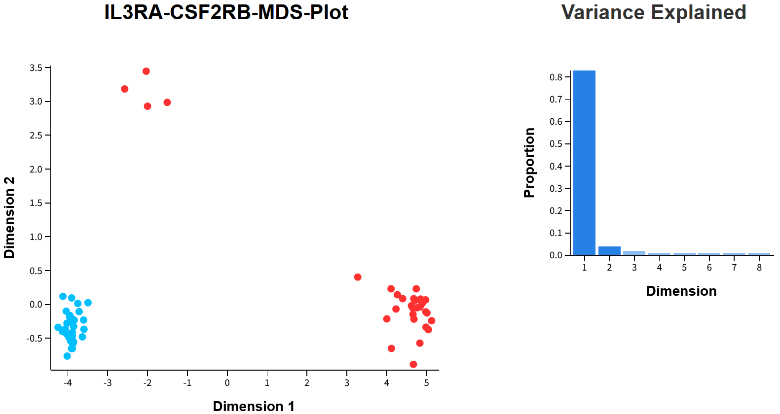
A few telling signs stand out. First, there is a huge near 90% explaining the separation between high (red) and low (blue) samples across dimension 1, something usually only observed between isogenic cell lines or technical replicates. Second, four samples from the high group appear not to belong? Diving into the GTEx metadata for the participants in these strata, we found that the RECOUNT3 GTEx Blood cohort had unaccounted substructure!
Below is the table of participants used in the above analysis separated by stratum. On the left is the low group (light blue background) with GTEx metadata showing consistently for each participant, membership in "GTEx SMTS Blood" and "GTEx SMTSD Whole Blood", as expected. On the right (light red background), the same for the high stratum showing that although all participants in this stratum are annotated as "GTEx SMTS Blood", the detailed annotation reveals all but four are actually "Cells - EBV-transformed lymphocytes". Unintentionally, we were comparing Whole Blood to EBV-transformed lymphocytes. (NOTE: “SMTS” - Tissue Type, area from which the tissue sample was taken and “SMTSD” - Tissue Type, more specific detail of tissue type)
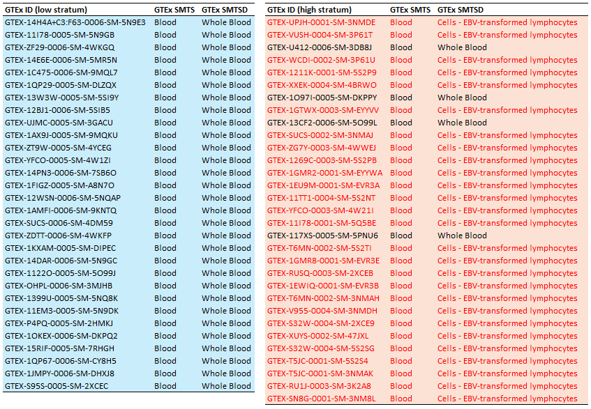
Undoubtedly, there is more substructure in the Whole Blood cohort, some subtle others maybe not?
10. Example commands
Single gene analysis
xxxxxxxxxx#1. RECOUNT3 - BRCA, ZEB1 High Vs Low, stratification threshold of 5%, DE onlyR3_analyse_GOI.sh -p BRCA -g ZEB1 -s mRNA -t 5 -d
#2. GTEx - Breast, ESR1 High Vs Low, stratification threshold of 7%, DE and correlation analysisGTEx_analyse_GOI.sh -p Breast -g ESR1 -s mRNA -t 7 -a
#3. GDC - TCGA-PRAD,  AR Low Vs High (switch comparison), stratification threshold of 3%, DE and correlation analysis, run GSEAGDC_TCGA_analyse_GOI.sh -p TCGA-PRAD -g AR -s mRNA -t 3 -S -a -e
Composite gene analysis - Additive mode
xxxxxxxxxx#1. RECOUNT3 - BREAST, ESR1-PGR-ERBB2 Low Vs High (switch comparison), stratification threshold of 6%, DE only, run GSEAR3_analyse_GOI.sh -p BREAST -g ESR1+PGR+ERBB2 -s mRNA -t 6 -S -d -e
#2. GDC - TCGA-KIRC, ZEB1-ESRP1 High Vs Low, stratification threshold of 10%, DE and correlation analysisGDC_TCGA_analyse_GOI.sh -p TCGA-KIRC -g ZEB1+ESRP1 -s mRNA -t 10 -a
Composite gene analysis - Ratio mode
xxxxxxxxxx#1. RECOUNT3 - LAML, IL3RA-CSF2RB High Vs Low, stratification threshold of 12%, DE only, run GSEAR3_analyse_GOI.sh -p LAML -g IL3RA%CSF2RB -s mRNA -t 12 -d -e
#2. GTEx - Breast, ESR1-PGR High Vs Low, stratification threshold of 2%, DE only, run GSEAGTEx_analyse_GOI.sh -p Breast -g ESR1%PGR -s mRNA -t 2 -d -e
Multimodal analysis
xxxxxxxxxx#1. GDC - TCGA-BRCA, hsa-miR-200c-3p High Vs Low, stratification threshold of 2%, DE only, run GSEAGDC_TCGA_analyse_GOI.sh -p TCGA-BRCA -g hsa-miR-200c-3p -s miRNA -t 2 -d -e
11. Custom Databases
11.1 Subsetting preconfigured DBs
TRANSECT comes with the capability of retrieving and formatting data from GTEx, GDC and RECOUNT3, ready for analyses. In some situations, there may be a strong case for refining or "subsetting" these data into smaller parts. At a bare minimum, TRANSECT requires 2 elements for each DB: 1. Count matrix and 2. TPM matrix. These matrices must be matching (identical dimensions with identical row and column names).
Here, we will use data from RECOUNT3 for TCGA-BRCA as an example of the steps required to initiate a subset-DB. We start in R, requiring the tidyverse and data.table R libraries. Once in R or RStudio, navigate to your RECOUNT3 BRCA data repository and execute the following code.
x
library(tidyverse)library(data.table)
### Navigate to the R3 BRCA data reposetwd("~/TRANSECT/data/RECOUNT3/BRCA") # modify this line to suit your setup### NOTE: If you dont have R3 BRCA yet, activate your TRANSECT environment and use the following command to retrieve it beforehand# conda activate TRANSECT# R3_prepare_directories.sh -p BRCA
### Next, we read from the BRCA clinical file, TCGA participant IDs and ESR1 receptor status. Take care to modify the clinical data file name in the following code appropriately as part of the name ("BRCA-2025-01-01") may be different for you compared to this examplebrca_esr1_dat <- fread("R3-BRCA-2025-01-01_clinical.tsv", select = c("tcga.gdc_cases.samples.portions.submitter_id","tcga.xml_breast_carcinoma_estrogen_receptor_status"), data.table = FALSE)## have a quick look at the resultshead(brca_esr1_dat)dim(brca_esr1_dat)table(brca_esr1_dat$tcga.xml_breast_carcinoma_estrogen_receptor_status)
### What we want now is a simple vector of all participant IDs whose estrogen receptor status is "Negative"esr1_neg_ids <- subset(brca_esr1_dat, tcga.xml_breast_carcinoma_estrogen_receptor_status == 'Negative')$tcga.gdc_cases.samples.portions.submitter_id## have a quick look at the resultsesr1_neg_ids## these IDs have an additional element at the end (last 3 characters) which TRANSECT does not use so we remove themesr1_neg_ids = substr(esr1_neg_ids,1,nchar(esr1_neg_ids)-3)## and finally, remove all duplictaesesr1_neg_ids <- unique(esr1_neg_ids)
### Next, use the list of IDs to retrieve only the count and TPM data for these participants from the expression tables### lets start with the count data. Take care to modify the count file name in the following code appropriately as it will be different to this examplebrca_esr1_neg_dat <- fread("R3-BRCA-2025-01-01_count-mRNA.tsv", select = c("gene_name",esr1_neg_ids), data.table = FALSE)## have a quick look at the resultshead(brca_esr1_neg_dat)dim(brca_esr1_neg_dat)
### If all looks good, lets save the subsetted table. The file name of the resulting table is important for TRANSECT### The parts of the file name that are important are the beginning ("R3-") and the end ("_count-mRNA.tsv" and/or "_tpm-mRNA.tsv")write.table(brca_esr1_neg_dat, "R3-BRCA_esr1-neg-2025-01-01_count-mRNA.tsv", sep='\t', row.names = FALSE)
### Now do the exact same for the TPM data. Again, take care to modify the tpm file name in the following code appropriately as it will be different to this examplebrca_esr1_neg_tpm_dat <- fread("R3-BRCA-2025-01-01_tpm-mRNA.tsv", select = c("gene_name",esr1_neg_ids), data.table = FALSE)dim(brca_esr1_neg_tpm_dat)write.table(brca_esr1_neg_tpm_dat, "R3-BRCA_esr1-neg-2025-01-01_tpm-mRNA.tsv", sep='\t', row.names = FALSE)
### Great, we have all we need (matching count and TPM tables) to setup a new DB for TRANSECT. ### These need to be housed in the same place as all the other DBs so we create a new parent folder. ### The name of the parent folder is important as this is what we will supply to TRANSECT - "BRCA-ESR1-neg"dir.create("~/TRANSECT/data/RECOUNT3/BRCA-ESR1-neg") # you will need to modify the directory path to suit your setup## Move the newly created tables to the new folder. Again, modify the directory path to suit your setupfile.rename(from="~/TRANSECT/data/RECOUNT3/BRCA/R3-BRCA_esr1-neg-2025-02-05_count-mRNA.tsv", to="~/TRANSECT/data/RECOUNT3/BRCA-ESR1-neg/R3-BRCA_esr1-neg-2025-02-05_count-mRNA.tsv")file.rename(from="~/TRANSECT/data/RECOUNT3/BRCA/R3-BRCA_esr1-neg-2025-02-05_tpm-mRNA.tsv", to="~/TRANSECT/data/RECOUNT3/BRCA-ESR1-neg/R3-BRCA_esr1-neg-2025-02-05_tpm-mRNA.tsv")
### Done! you should now have a folder in TRANSECT/data/RECOUNT3/ called BRCA-ESR1-neg that contains two matching files, one for count data and the other for TPMs. Feel free to exit out of your R session now.Next, we open a bash terminal and execute the following commands
xxxxxxxxxx### Now that we have a new DB folder, we first need to add it to the TRANSECT list of known DBs### These can be found in the TRANSECT top directory in "REF_FILES/study_abbreviations". The full path to this folder will be different for you so ammend the following code appropriately### NOTE: there is a single file for each: RECOUNT3, GTEx and GDC. Make sure when you do this type of thing that you modify the appropriate file!echo -e 'BRCA-ESR1-neg\tCustom' >> /home/jtoubia/TRANSECT/REF_FILES/study_abbreviations/R3_Study_Abbreviations.tsv
### Activate the TRANSECT environment (if not already done) and navigate to an appropriate output folderconda activate TRANSECTcd /home/jtoubia/TRANSECT/output/RECOUNT3/ # ammend this path to suit your setup
### Lets create a new folder for this test runmkdir Custom_DB_Trialcd Custom_DB_Trial
### Time to run TRANSECT. Remember, we created a RECOUNT3 DB and housed it in the R3 DB folder, so we need to use the R3 TRANSECT script in order for this to work### We know that PGR is mostly off when ESR1 is absent so lets try ERBB2### We want TRANSECT to use our new custom DB so we need to pass this info using the -p parameterR3_analyse_GOI.sh -p BRCA-ESR1-neg -g ERBB2 -s mRNA -t 10 -d
Done! The same procedure can be used for subsetting any other DB from each of the three data sources. Just remember to abide by the appropriate naming conventions and be consistent when applying this name to the TRANSECT/REF_FILES/study_abbreviations/ documents.
11.2 Using private, in-house or custom data sets
Private, in-house and custom data can be likewise configured if the reference genome used to create the matrix is the same as what TRANSECT uses (gencode v36 for GDC; v26:v39 for GTEx and; v26 for R3). In cases where this in not true, extra steps are required. Let's start from the beginning.
Open a bash terminal and execute the following commands
x
### First thing we need is appropriate data. For demonstration purposes, I've chosen gene expression data from the Pediatric Brain Tumor Atlas (CBTTC) cohort hosted on UCSC Xena. See https://xenabrowser.net/datapages/?cohort=Pediatric%20Brain%20Tumor%20Atlas%3A%20CBTTC&removeHub=https%3A%2F%2Fxena.treehouse.gi.ucsc.edu%3A443### This cohort is large (n=973) and has downloadable counts and TPM data in the right format - ROWs (identifiers) x COLUMNs (samples) (i.e. genomicMatrix). ### However as you will soon see, it requires a little effort to make it work in TRANSECT and forms a good example of some of the hurdles that one might face.
### To start, get the data and put in in an appropriate directory. For custom analyses like these, I recomend using the RECOUNT3 TRANSECT pipeline.### Navigate to the R3 data repo and create a new foldercd ~/TRANSECT/data/RECOUNT3/ # modify this line to suit your setupmkdir XENA_PBTA # this is what we we call the DB but it could be anything as long as we are consistentcd XENA_PBTA/
### Get the data and unpackwget https://kidsfirstxena.s3.us-east-1.amazonaws.com/download/CBTTC%2FCBTTC_rsem.genes_expected_count.txt.gzwget https://kidsfirstxena.s3.us-east-1.amazonaws.com/download/CBTTC%2FCBTTC_rsem.genes_TPM.txt.gzgunzip CBTTC%2FCBTTC_rsem.genes_expected_count.txt.gzgunzip CBTTC%2FCBTTC_rsem.genes_TPM.txt.gzWe will come back to this terminal but need now to swap over into R for some data wrangling.
x
### In R or RStudio, load libraries and go to the new directorylibrary(tidyverse)library(data.table)library(tibble)
setwd("~/TRANSECT/data/RECOUNT3/XENA_PBTA") # modify this line to suit your setup
### Read in the datacount_dat <- fread("CBTTC%2FCBTTC_rsem.genes_expected_count.txt", sep="\t", data.table = FALSE)tpm_dat <- fread("CBTTC%2FCBTTC_rsem.genes_TPM.txt", sep="\t", data.table = FALSE)
### Quick integrity checks on the two files (which looks good at first sight)dim(count_dat)dim(tpm_dat)### Quick look at the datacount_dat[1:5,1:5]tpm_dat[1:5,1:5]
### A few things to note. The dimension of both tables are the same which is great. ### This does not necessarily mean that the row and column names are identical but they are. Always check.### Turns out however, that there are columns with duplicate names!### The gene_id's are formed by using a combination of ENSEMBL IDs and gene names, not what TRANSECT expects. ### Also, TRANSECT expects the ID column to be named "gene_name"### And finally, the data is transformed: Counts = log2(expected_count+1) and, TPM = log2(TPM+0.001).
### Step 1. deduplicate columnscount_dat <- count_dat[, !duplicated(colnames(count_dat))]tpm_dat <- tpm_dat[, !duplicated(colnames(tpm_dat))]dim(count_dat)dim(tpm_dat)
### Step 2. gene_id's are in a column which makes working on the matrix slightly harder. Move the gene_id column to indexcount_dat <- count_dat %>% column_to_rownames('gene_id')tpm_dat <- tpm_dat %>% column_to_rownames('gene_id')
### Step 3. reverse the transformationcount_dat <- 2^count_dat-1tpm_dat <- 2^tpm_dat-0.001
### Step 4. move rownames back and assign the new column namecount_dat <- rownames_to_column(count_dat, "gene_name")tpm_dat <- rownames_to_column(tpm_dat, "gene_name")
### Step 5. Save to filewrite.table(count_dat %>% mutate_if(is.numeric, round, digits=2), "R3-XENA_PBTA-2025-02-05_count-mRNA.tsv", sep='\t', row.names = FALSE)write.table(tpm_dat %>% mutate_if(is.numeric, round, digits=2), "R3-XENA_PBTA-2025-02-05_tpm-mRNA.tsv", sep='\t', row.names = FALSE)
### Done! you should now have a folder in TRANSECT/data/RECOUNT3/ called XENA_PBTA that contains two matching files, one for count data and the other for TPMs. For now, don't exit out of your R session, we will be back.Next, we go back to the bash terminal and execute the following commands
x
### Now that we have a new DB, like in section 11.1, we first need to add it to the TRANSECT list of known DBs### These can be found in the TRANSECT top directory in "REF_FILES/study_abbreviations". The full path to this folder will be different for you so ammend the following code appropriately### NOTE: there is a single file for each: RECOUNT3, GTEx and GDC. Make sure when you do this type of thing that you modify the appropriate file!echo -e 'XENA_PBTA\tCustom' >> /home/jtoubia/TRANSECT/REF_FILES/study_abbreviations/R3_Study_Abbreviations.tsv
### Activate the TRANSECT environment (if not already) and navigate to an appropriate output folderconda activate TRANSECTcd /home/jtoubia/TRANSECT/output/RECOUNT3/ # ammend this path to suit your setup
### Lets create a new folder for this test runmkdir Custom_DB_Trial2cd Custom_DB_Trial2
### Time to run TRANSECT. Remember, we created a RECOUNT3 DB and housed it in the R3 DB folder, so we need to use the R3 TRANSECT script in order for this to work### We will assess disparate expression of the gene QKI. Seeing this is a large DB (n=973), we choose a small stratifictaion threshold of 3.### We want TRANSECT to use our new custom DB so we need to pass this info using the -p parameterR3_analyse_GOI.sh -p XENA_PBTA -g QKI -s mRNA -t 3 -d
### If everything worked, the pipeline should fail! The error, "object 'QKI' not found".### TRANSECT is looking for the exact and complete text "QKI" in the gene_name column of the expression matrix but, it is not there.### Lets look for itcut -f 1 ~/TRANSECT/data/RECOUNT3/XENA_PBTA/R3-XENA_PBTA-2025-02-05_count-mRNA.tsv | grep "QKI"
### and we get "ENSG00000112531.16_QKI". This is what we need to provide to TRANSECT however, there is another issue.### by default, TRANSECT checks if the user provided a legitimate gene ID. If we try and pass "ENSG00000112531.16_QKI" in the command above this will fail too. Try it.### Instead, we need to tell TRANSECT not to check gene names by passing the -x parameterR3_analyse_GOI.sh -p XENA_PBTA -g ENSG00000112531.16_QKI -s mRNA -t 3 -d -x
### Voila!Stratification and DE work. If this is all you need then job done!
But, both WebGestalt and GSEA expect actual gene names and will complain about the likes of "ENSG00000112531.16_QKI". If these analyses are required then, back into R to fix the issue.
x
### Navigate back to the R3 data reposetwd("~/TRANSECT/data/RECOUNT3/XENA_PBTA") # modify this line to suit your setup
### Load libraries if this is a new sessionlibrary(tidyverse)library(data.table)
### Read in the data. Start with the count datacount_dat <- fread("R3-XENA_PBTA-2025-02-05_count-mRNA.tsv", sep="\t", data.table = FALSE)
### Modify gene names and check for duplicate valuescount_dat$gene_name <- unlist(lapply(strsplit(as.character(count_dat$gene_name), "_"), '[[', 2))n_occur <- data.frame(table(count_dat$gene_name))n_occur[n_occur$Freq > 1,]
### It turns out that after removing ENSEMBL IDs, 254 elements have more than 1 row in the data table (some have hundreds!).### Because TRANSECT uses this column as an index, it will crash if duplicates are present, we need to remove them.### There are many options here, all come with consequences. A description of each with pros and cons is out of scope here, you need to decide how best to handle this issue for your situation.### NOTE: because only 254 genes are dups and because most of these are rRNAs, lincs, snords, ...., you may except the loss and remove all of them?### For demo purposes, we will just blindly deduplicate.count_dat <- count_dat[!duplicated(count_dat$gene_name), ]
### Finally we can save the tablewrite.table(count_dat, "R3-XENA_PBTA-2025-02-05_count-mRNA.tsv", sep='\t', row.names = FALSE)
### We need to do the same for the tpm data.tpm_dat <- fread("R3-XENA_PBTA-2025-02-05_tpm-mRNA.tsv", sep="\t", data.table = FALSE)tpm_dat$gene_name <- unlist(lapply(strsplit(as.character(tpm_dat$gene_name), "_"), '[[', 2))tpm_dat <- tpm_dat[!duplicated(tpm_dat$gene_name), ]write.table(tpm_dat, "R3-XENA_PBTA-2025-02-05_tpm-mRNA.tsv", sep='\t', row.names = FALSE)And, finally... (I promise :-), we can run TRANSECT to completion.
x
### Back in the terminalR3_analyse_GOI.sh -p XENA_PBTA -g QKI -s mRNA -t 3 -d -x
### Note, because the gene_name QKI is known to TRANSECT, we don't actually require the -x parameter but that will not be the case for all gene names in this DB.
### One last thing, we still have the raw PBTA data and these files are large (and no longer required). They can be deletedrm /home/jtoubia/TRANSECT/data/RECOUNT3/XENA_PBTA/CBTTC%2FCBTTC_rsem.genes_expected_count.txtrm /home/jtoubia/TRANSECT/data/RECOUNT3/XENA_PBTA/CBTTC%2FCBTTC_rsem.genes_TPM.txtAnd, that's it! A few things to consider if you decide to venture into something like this;
Be prepared, you will likely have to do some major data wrangling, a good Data Scientist/bioinformatician goes a long way.
Some data sets are extremely large and equally unwieldy. Be prepared.
Because TRANSECT is configured to recognise TCGA and GTEx participant identifiers, when using these data TRANSECT knows which samples are cancer and which are not ("normal"). For custom DBs with unknown/unrecognisable participant/sample IDs, TRANSECT will not know whether these are diseased or not, whether they are human or not, whether the data is expression or not. In these cases, the plots produced will all default to "normal" samples and "TPM" measurements, whether this is true or not.
12. Publication details
Currently unpublished.
![]() This manual was produced in markdown using typora v1.9.5
This manual was produced in markdown using typora v1.9.5